
Don't want to miss a thing?
Efficiently Detect Corrosion with SoftServe’s Visual Inspection Solution
Last updated: 31.07.2025
Visual inspection is indispensable in the oil and gas industry and manufacturing. Industries in which meticulous scrutiny of structures, equipment, and processes is essential for operational integrity, safety compliance, and quality assurance.
Technological advancements make integrating sophisticated inspection methodologies to enhance efficiency and minimize risks in these high-stakes environments necessary. Artificial intelligence (AI) has emerged as a transformative force in the evolving visual inspection landscape, leveraging machine learning (ML) for more accurate and efficient corrosion detection.
Integrating AI accelerates detection speed and reduces error margins. It also offers a level of precision beyond traditional methods. The potential combination of drones and AI in visual inspection holds immense promise by capturing high-resolution images in challenging locations and enabling swift, accurate identification of structural issues, defects, or anomalies.
Our project and the dataset
We leveraged our extensive data annotation and model performance analysis experience to create an effective corrosion detection solution. This solution uses segmentation in a supervised setting and maximizes a limited dataset.
As a result, we developed a versatile, lightweight corrosion detection model that can be deployed across various settings, including both cloud and edge environments. This scalable model also paves the way to potentially detect other anomalies in the future.
To train and tune the models, we used a “corrosion image dataset for automating scientific assessment of materials.” This novel dataset comprises 600 images annotated with expert corrosion ratings that have been accumulated during more than a decade of laboratory testing by material scientists. It aims to address the lack of standardized experimental data in the public domain for developing machine learning models in corrosion research, a field that significantly impacts global expenses and safety. This kind of annotated data also supports the development of corrosion modelling software by providing real-world benchmarks for predictive tools.
During the preparation phase, we manually labeled 183 images and obtained an initial supervised dataset for model tuning. However, the challenge remained of addressing little background variety, which we solved by using a custom data augmentation. We’ll describe that further in this article.
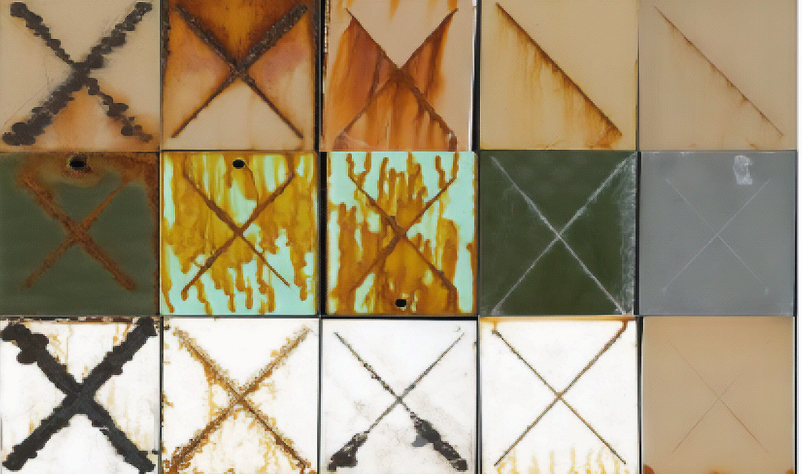
Figure 1. Sample images from the dataset
To address the extremely scarce amount of labeled data, we applied a set of standard and custom augmentations to increase the amount of available data. We applied random crops of fixed size, randomly sized crops, Gaussian blur, and noise to the images and applied random grid shuffles.
A. RandomCrop(height=128, width=128, p=0.7)

B. OneOf(transforms=[A.GaussianBlur(blur_limit=(3, 7), sigma_limit=0, p=1),

A.GaussNoise(var_limit=(10, 50), mean=0, per_channel=True, p=1)], p=1)

C.RandomGridShuffle(grid=(3, 3), p=1)
On top of that, we added coarse, grid and mask dropouts, elastic transformations, and optical distortions.
A. OneOf(

transforms=[

A.CoarseDropout(

max_holes=3,

max_height=0.5,

max_width=0.5,

min_holes=1,

min_height=0.1,

min_width=0.1,

fill_value=0,

mask_fill_value=0,

p=1,

),

A.GridDropout(

ratio=0.5,

holes_number_x=3,

holes_number_y=3,

random_offset=True,

fill_value=0,

mask_fill_value=0,

p=1,

),

B. MaskDropout(max_objects=(1, 3),

image_fill_value= mask_fill_value=0,

p=1),

],

p=0.5,

)
Finally, we applied affine and flip transformations, rotations, and transpositions.
A. One Of (

transforms=[

A.Affine( (

Scale = 0, # (0.75, 1.25)

translate percent = (-0.25, 0.25),

rotate = (-180, 180),

shear = (-45, 45),

interpolation = cv.INTER_LINEAR,

mask interpolation = cv. INTER_NEAREST,

cval=0,

cval_mask=0,

mode=cv.BORDER_REFLECT,

keep_ratio=True,

p=1,

),

B. ElasticTransform(

alpha=5000,

sigma=50,

alpha_affine=0,

interpolation=cv.INTER_LINEAR,

border_mode=cv.BORDER_REFLECT,

value=None,

mask_value=None,

p=1,

),

C. GridDistortion(

num_steps=5,

distort_limit=(-0.3, 0.3),

interpolation=cv.INTER_LINEAR,

border_mode=cv.BORDER_REFLECT,

value=None,

mask_value=None,

p=1,

),

D. OpticalDistortion(

distort_limit=(-0.3, 0.3),

shift_limit=(-0.05, 0.05),

interpolation=cv.INTER_LINEAR,

border_mode=cv.BORDER_REFLECT,

value=None,

mask_value=None,

p=1,

),

],

p=0.5,

)
These augmentations all address the variety of materials, angles and images, and distortions of corrosion images in the real world.
However, the main problem with the available dataset was in the relatively poor variety of backgrounds on the images. To solve this problem, we implemented custom augmentation that could replace the background class pixels with different values and apply other backgrounds. This augmentation was a huge deal-breaker in generalizing the model on a diverse dataset.

Figure 2. Applications of custom background replacement augmentation
The model
For model architecture, we conducted a series of experiments and concluded that U-Net++ architecture with MobileNetV2 as a backbone and a depth level of five presented the best balance between performance and accuracy.
U-Net++ presents a series of improvements over standard U-Net architecture:
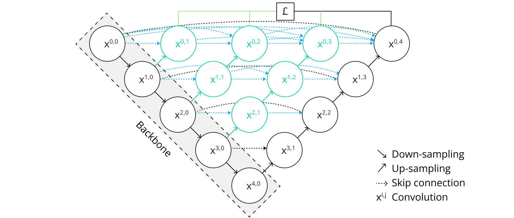
Figure 3. U-Net++ architecture
U-Net++ provides a series of nested, dense skip pathway connections. Their goal is to bridge the semantic gap between the feature maps of the encoder and decoder more effectively. This results in better feature propagation and fusion, leading to more precise segmentation results.
The architecture selection was made to support both edge and cloud deployment and the selected architecture demonstrated satisfactory performance on the evaluation dataset. Moreover, “heavier” models are prone to overfitting on such a small dataset and are impractical for the current problem.
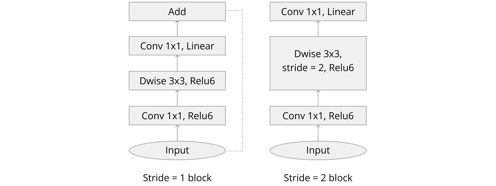
MobileNetV2 is an excellent choice for this case, as it also has a set of pre-trained models to accelerate the tuning process. It features lightweight architecture with inverted residuals. The expansion layer uses depth-wise separable convolutions to filter features as a source of non-linearity.
The training and evaluation setup
As mentioned earlier, we used a batch size of 32 and trained the model during 90 epochs. The training was stopped when the delta on model improvements was insignificant for recent epochs. The model was trained using Focal loss and Adam optimizer, with a weight decay of 0.001. To address the model learning curve, we applied a learning rate scheduler that reduced the learning rate on the metric plateau.
The performance of the model was evaluated mainly using intersection over union (IoU) or Jaccard Index and Dice metrics.

The results
After a series of experiments, we selected a model for evaluation, and it presented sufficient results on the hold-out data, which even exceeded the validation results a bit.

Examples of how the model predicts corrosion and stains are presented below.
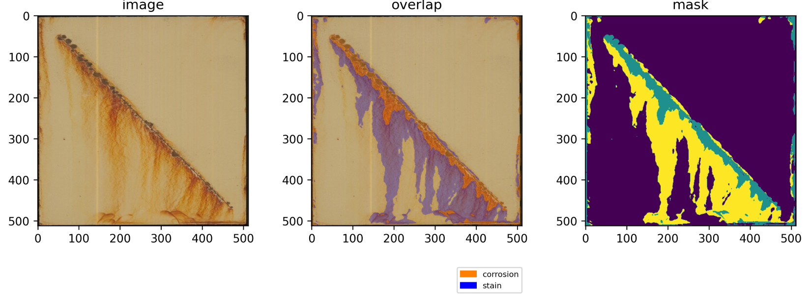
Figure 5. Model performance comparison with ground truth data
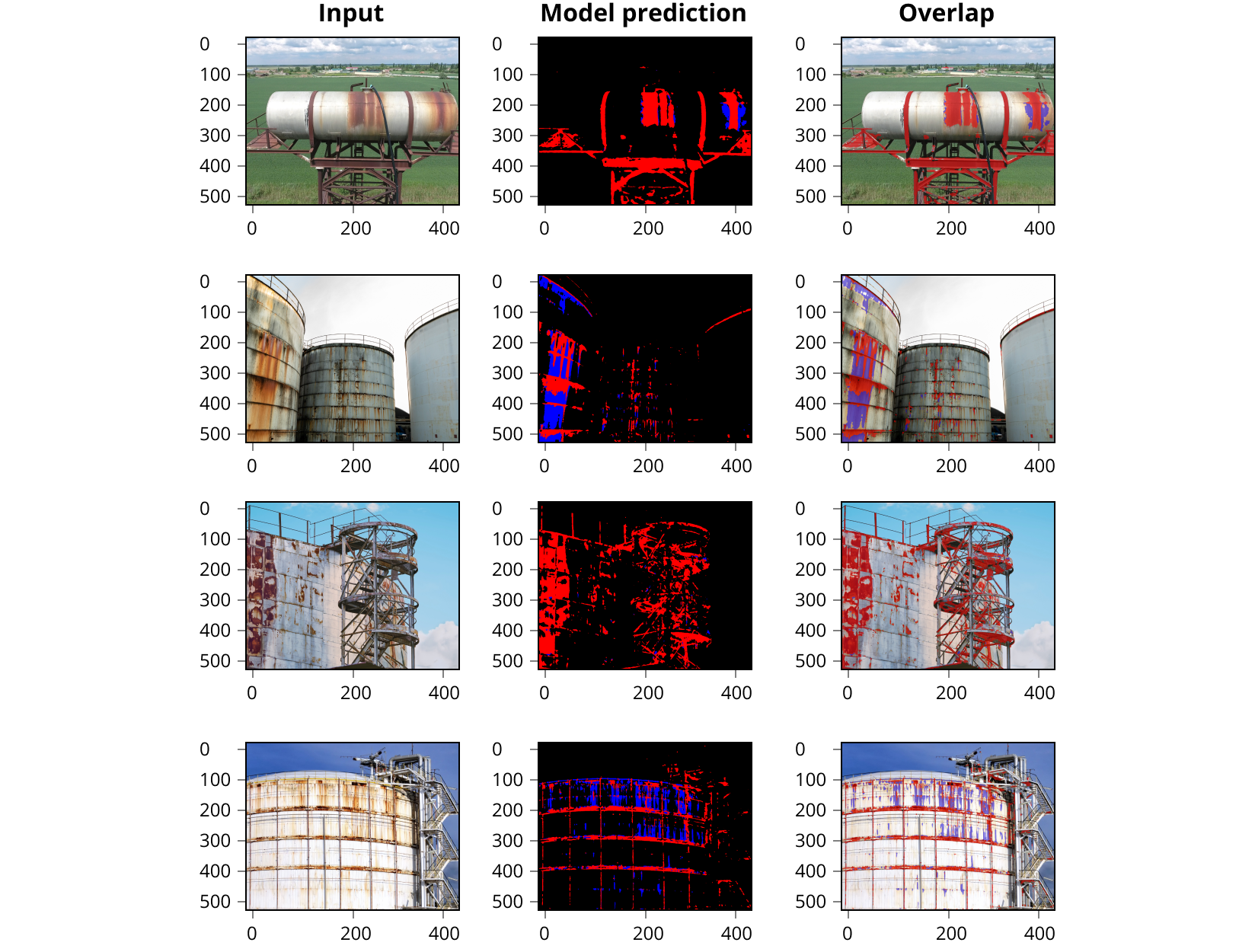
Also, the model was tested on real-world images that did not come from the original data distribution.
Conclusion
SoftServe’s corrosion detection solution is a paradigm shift in visual inspection within the oil and gas and manufacturing industries.
Our approach, which used segmentation in a supervised setting, resulted in a solution that’s adaptable in various settings. Overcoming the challenge of limited background variety, we implemented custom augmentation techniques that showcase our commitment to innovation.
We also used U-Net++ architecture that was paired with MobileNetV2 encoder, which is an excellent balance of power and efficiency.
One of our main areas of research and development was processing an open-source dataset, which we enriched and augmented to better suit our needs. Advanced augmentations allowed for much better real-world performance.
The project’s results exceeded our expectations on hold-out data and real-world images, demonstrating the solution’s effectiveness and resilience in real-world applications.
In this transformative journey, we not only detect corrosion but redefine visual inspection. By contributing to the broader landscape of AI corrosion control, our solution helps industrial teams act early and more precisely.

